Imports
%%capture
!pip install deepface
import cv2
import random
import numpy as np
import matplotlib.pyplot as plt
import matplotlib.patches as patches

from deepface import DeepFace
from tqdm import tqdm
from skimage import data
from sklearn.cluster import KMeans
from sklearn.svm import SVC
from sklearn.preprocessing import StandardScaler
from sklearn.model_selection import train_test_split
from sklearn.metrics import classification_report, accuracy_score
from tensorflow.keras.datasets import cifar10
24-09-19 14:18:07 - Directory /root/.deepface has been created
24-09-19 14:18:07 - Directory /root/.deepface/weights has been created
2D Planar Transformations

In this section, we explore how to map points from one 2D coordinate system to another. These transformations are the mathematical foundation for image warping, image registration (aligning two images), and creating panoramas.
We categorize these transformations based on their Degrees of Freedom (DOF) and what geometric properties they preserve (Invariants).
The Hierarchy of Transformations
Richard Szeliski's Computer Vision: Algorithms and Applications defines a hierarchy of transformations. As we move down the list, the transformation becomes more powerful but preserves fewer properties.
- Translation: Shifting position only.
- Euclidean (Rigid): Translation + Rotation.
- Similarity: Translation + Rotation + Uniform Scale.
- Affine: Shear and non-uniform scaling (parallel lines stay parallel).
- Projective (Homography): Perspective distortion (lines stay straight, but parallel lines converge).
Mathematical Prerequisite: Homogeneous Coordinates
In the code below, you will see us converting 2D points $(x, y)$ into 3D vectors $(x, y, 1)$. Why?
A standard $2 \times 2$ matrix multiplication can calculate rotation and scaling, but it cannot calculate translation (shifting points). To represent translation as a matrix multiplication (which allows us to chain transformations using dot products), we increase the dimension by one.
$$ \begin{bmatrix} x' \\ y' \\ 1 \end{bmatrix} = \begin{bmatrix} r_{00} & r_{01} & t_x \\ r_{10} & r_{11} & t_y \\ 0 & 0 & 1 \end{bmatrix} \cdot \begin{bmatrix} x \\ y \\ 1 \end{bmatrix} $$
1. Translation
Translation is the simplest transformation. It simply moves every point by a fixed distance $(t_x, t_y)$.
- Degrees of Freedom (DOF): 2 ($t_x, t_y$)
- Preserves: Orientation, lengths, angles, parallelism, and straight lines.
The Matrix: The identity matrix with an offset in the last column. $$ H_t = \begin{bmatrix} 1 & 0 & t_x \\ 0 & 1 & t_y \\ 0 & 0 & 1 \end{bmatrix} $$
# Translation: Moves every point of an object by the same distance in a given direction.
def plot_translation():
    # Original shape: a square
    square = np.array([[1, 1], [1, 3], [3, 3], [3, 1], [1, 1]])

    # Translation matrix (tx = 2, ty = 1)
    tx, ty = 2, 1
    T = np.array([[1, 0, tx],
                  [0, 1, ty],
                  [0, 0, 1]])

    # Homogeneous coordinates
    square_homogeneous = np.c_[square, np.ones((square.shape[0], 1))]

    # Apply translation
    translated_square = (T @ square_homogeneous.T).T[:, :2]

    # Plot original and translated squares
    plt.figure(figsize=(6, 6))
    plt.plot(square[:, 0], square[:, 1], 'b-', label='Original')
    plt.plot(translated_square[:, 0], translated_square[:, 1], 'r-', label='Translated')
    plt.title('Translation Transformation')
    plt.axis('equal')
    plt.legend()
    plt.show()

plot_translation()

2. Euclidean (Rigid) Transformation
Also known as a "Rigid Body Transform." Imagine throwing a cardboard square across a table. It can move (translate) and turn (rotate), but it cannot stretch or bend.
- Degrees of Freedom: 3 (1 Rotation angle $\theta$ + 2 Translation).
- Preserves: Lengths (isometric) and Areas.
The Matrix: The top-left $2 \times 2$ submatrix is a standard 2D rotation matrix $R$. $$ H_e = \begin{bmatrix} \cos\theta & -\sin\theta & t_x \\ \sin\theta & \cos\theta & t_y \\ 0 & 0 & 1 \end{bmatrix} $$
# Euclidean (Rigid): Combines rotation and translation, preserving distances and angles.
def plot_euclidean():
    # Original shape: a square
    square = np.array([[1, 1], [1, 3], [3, 3], [3, 1], [1, 1]])

    # Rotation matrix for 45 degrees
    theta = np.radians(45)
    R = np.array([[np.cos(theta), -np.sin(theta), 0],
                  [np.sin(theta), np.cos(theta), 0],
                  [0, 0, 1]])

    # Translation matrix (tx = 2, ty = 1)
    tx, ty = 2, 1
    T = np.array([[1, 0, tx],
                  [0, 1, ty],
                  [0, 0, 1]])

    # Combined Euclidean transformation (Translation + Rotation)
    Euclidean = T @ R

    # Homogeneous coordinates
    square_homogeneous = np.c_[square, np.ones((square.shape[0], 1))]

    # Apply Euclidean transformation
    transformed_square = (Euclidean @ square_homogeneous.T).T[:, :2]

    # Plot original and transformed squares
    plt.figure(figsize=(6, 6))
    plt.plot(square[:, 0], square[:, 1], 'b-', label='Original')
    plt.plot(transformed_square[:, 0], transformed_square[:, 1], 'r-', label='Euclidean (Rigid)')
    plt.title('Euclidean (Rigid) Transformation')
    plt.axis('equal')
    plt.legend()
    plt.show()

plot_euclidean()

3. Similarity Transformation
A similarity transform includes translation, rotation, and a uniform scale factor ($s$). The object changes size, but its "shape" remains identical.
- Degrees of Freedom: 4 (1 Scale $s$ + 1 Rotation $\theta$ + 2 Translation).
- Preserves: Angles (conformal) and ratios of lengths. (e.g., a square remains a square, just larger or smaller).
The Matrix: $$ H_s = \begin{bmatrix} s\cos\theta & -s\sin\theta & t_x \\ s\sin\theta & s\cos\theta & t_y \\ 0 & 0 & 1 \end{bmatrix} $$
# Similarity: Combines Euclidean transformations with scaling, preserving the shape.
def plot_similarity():
    # Original shape: a square
    square = np.array([[1, 1], [1, 3], [3, 3], [3, 1], [1, 1]])

    # Rotation matrix for 30 degrees
    theta = np.radians(30)
    R = np.array([[np.cos(theta), -np.sin(theta), 0],
                  [np.sin(theta), np.cos(theta), 0],
                  [0, 0, 1]])

    # Scaling factor
    s = 1.5
    S = np.array([[s, 0, 0],
                  [0, s, 0],
                  [0, 0, 1]])

    # Translation matrix (tx = 2, ty = 1)
    tx, ty = 2, 1
    T = np.array([[1, 0, tx],
                  [0, 1, ty],
                  [0, 0, 1]])

    # Combined Similarity transformation (Translation + Rotation + Scaling)
    Similarity = T @ R @ S

    # Homogeneous coordinates
    square_homogeneous = np.c_[square, np.ones((square.shape[0], 1))]

    # Apply Similarity transformation
    transformed_square = (Similarity @ square_homogeneous.T).T[:, :2]

    # Plot original and transformed squares
    plt.figure(figsize=(6, 6))
    plt.plot(square[:, 0], square[:, 1], 'b-', label='Original')
    plt.plot(transformed_square[:, 0], transformed_square[:, 1], 'r-', label='Similarity')
    plt.title('Similarity Transformation')
    plt.axis('equal')
    plt.legend()
    plt.show()

plot_similarity()

4. Affine Transformation
Affine transformations allow for shearing and non-uniform scaling (scaling $x$ differently than $y$). This approximates looking at a flat object from a distance, where perspective effects are negligible.
- Visualizing it: A rectangle can become a parallelogram.
- Degrees of Freedom: 6 (The top two rows can be any numbers).
- Preserves: Parallelism. Parallel lines remain parallel after transformation. (Note: Angles and lengths are not preserved).
The Matrix: $$ H_a = \begin{bmatrix} a_{00} & a_{01} & t_x \\ a_{10} & a_{11} & t_y \\ 0 & 0 & 1 \end{bmatrix} $$
# Affine: A general linear transformation that includes scaling, rotation, translation, and shearing,
# preserving parallelism but not necessarily distances or angles.
def plot_affine():
    # Original shape: a square
    square = np.array([[1, 1], [1, 3], [3, 3], [3, 1], [1, 1]])

    # Affine transformation matrix (rotation, scaling, shearing, translation)
    A = np.array([[1, 0.5, 1],   # Shear + Scale + Translate
                  [0.5, 1, 1],
                  [0, 0, 1]])

    # Homogeneous coordinates
    square_homogeneous = np.c_[square, np.ones((square.shape[0], 1))]

    # Apply Affine transformation
    transformed_square = (A @ square_homogeneous.T).T[:, :2]

    # Plot original and transformed squares
    plt.figure(figsize=(6, 6))
    plt.plot(square[:, 0], square[:, 1], 'b-', label='Original')
    plt.plot(transformed_square[:, 0], transformed_square[:, 1], 'r-', label='Affine')
    plt.title('Affine Transformation')
    plt.axis('equal')
    plt.legend()
    plt.show()

plot_affine()

5. Projective Transformation (Homography)
This is the most general planar transformation. It models perspective distortion. This is what happens when you take a picture of a square tile floor from an angle; the tiles closer to you look large, and the tiles further away look small.
- Visualizing it: A square can become an arbitrary quadrilateral.
- Degrees of Freedom: 8 (The matrix has 9 numbers, but the scale is arbitrary, so we fix the last element to 1, leaving 8 variables).
- Preserves: Straight Lines (collinearity). Parallel lines may converge towards a vanishing point.
The Matrix & Normalization: Notice the bottom row is no longer $[0, 0, 1]$. It is $[h_{20}, h_{21}, 1]$. This introduces a $w'$ term in the result vector: $[x', y', w']$. To get back to 2D Cartesian coordinates, we must perform Perspective Division: $$x_{final} = \frac{x'}{w'}, \quad y_{final} = \frac{y'}{w'}$$
$$ H_p = \begin{bmatrix} h_{00} & h_{01} & h_{02} \\ h_{10} & h_{11} & h_{12} \\ h_{20} & h_{21} & 1 \end{bmatrix} $$
# Projective: A transformation that applies perspective distortion, which can map a square to any
# quadrilateral, preserving straight lines but not parallelism.
def plot_projective():
    # Original shape: a square
    square = np.array([[1, 1], [1, 3], [3, 3], [3, 1], [1, 1]])

    # Projective transformation matrix
    P = np.array([[1, 0.2, 0.5],
                  [0.3, 1, 0.5],
                  [0.001, 0.001, 1]])  # Perspective effect

    # Homogeneous coordinates
    square_homogeneous = np.c_[square, np.ones((square.shape[0], 1))]

    # Apply Projective transformation
    transformed_square = (P @ square_homogeneous.T).T
    transformed_square /= transformed_square[:, 2].reshape(-1, 1)  # Normalize by the third coordinate

    # Plot original and transformed squares
    plt.figure(figsize=(6, 6))
    plt.plot(square[:, 0], square[:, 1], 'b-', label='Original')
    plt.plot(transformed_square[:, 0], transformed_square[:, 1], 'r-', label='Projective')
    plt.title('Projective Transformation')
    plt.axis('equal')
    plt.legend()
    plt.show()

plot_projective()

Lens Distortions
So far, we have assumed a perfect Pinhole Camera Model, where light rays travel in perfectly straight lines through a microscopic aperture. In the real world, however, we use Lenses to gather more light.
The Physics of Imperfection
Lenses are curved pieces of glass. While they allow us to capture bright images, they introduce Radial Distortion. This means that straight lines in the real world (like the edge of a building) appear curved in the image.
The Brown-Conrady Model
In Computer Vision, we model this distortion mathematically so we can correct it (Calibration). The most common model describes the displacement of a pixel based on its distance $r$ from the optical center (principal point).
If $(x, y)$ are the ideal (undistorted) normalized coordinates, and $(x_{dist}, y_{dist})$ are the distorted coordinates, the relationship is modeled by a polynomial series:
$$x_{dist} = x (1 + k_1 r^2 + k_2 r^4 + k_3 r^6 + \dots)$$ $$y_{dist} = y (1 + k_1 r^2 + k_2 r^4 + k_3 r^6 + \dots)$$
Where:
- $r^2 = x^2 + y^2$ (Squared radial distance).
- $k_1, k_2, k_3$ are the Distortion Coefficients.

1. Visualizing Distortion: The Checkerboard
To detect lens distortion, we need a reference object with known straight lines. A Checkerboard (or chessboard) is the standard calibration target in Computer Vision because:
- It has high-contrast corners that are easy to detect automatically.
- It creates a strict grid of straight lines.
If we look at a checkerboard through a distorted lens, the straight grid lines will appear bent.
# Function to generate a checkerboard pattern
def generate_checkerboard(size=8, num_tiles=8):
    # Create an alternating black and white pattern
    row_pattern = np.array([0, 1] * num_tiles)
    checkerboard = np.row_stack([row_pattern, row_pattern[::-1]] * num_tiles)

    # Scale up the checkerboard pattern to desired size
    checkerboard = np.kron(checkerboard, np.ones((size, size)))

    # Convert to RGB format for OpenCV/Matplotlib (checkerboard is initially black & white)
    checkerboard_rgb = np.stack([checkerboard] * 3, axis=-1) * 255  # Convert to 3-channel RGB and scale to 255
    return checkerboard_rgb.astype(np.uint8)

# Generate the checkerboard image
checkerboard_image = generate_checkerboard(size=50, num_tiles=27)

# Display the checkerboard image
plt.imshow(checkerboard_image)
plt.title('Checkerboard Image')
plt.axis('off')
plt.show()

In the code below, we simulate the three most common manifestations of radial distortion by manipulating the coefficients $k_1, k_2,$ and $k_3$.
A. Barrel Distortion ($k_1 > 0$)
This typically occurs in wide-angle lenses and action cameras (like GoPros).
- Visual Effect: Straight lines bulge outward at the center, like the sides of a barrel.
- Cause: Magnification decreases as the distance from the optical center increases. The image gets "squashed" at the edges.
B. Pincushion Distortion ($k_1 < 0$)
This is common in telephoto (zoom) lenses.
- Visual Effect: Straight lines bow inward, as if the image is being pinched toward the center.
- Cause: Magnification increases with the distance from the optical center. The corners are stretched out.
C. Complex / Mustache Distortion
Real lenses sometimes exhibit a mix of both. For example, a lens might have barrel distortion near the center ($k_1 > 0$) but pincushion distortion at the far edges ($k_2 < 0$). This results in "wavy" lines that resemble a mustache.
def distort_image(image, k1=0, k2=0, k3=0):
    h, w = image.shape[:2]
    fx, fy = 0.9 * w, 0.9 * h  # Focal length
    cx, cy = w / 2, h / 2  # Center of the image

    # Camera matrix
    camera_matrix = np.array([[fx, 0, cx],
                              [0, fy, cy],
                              [0, 0, 1]], dtype=np.float32)

    # Distortion coefficients
    dist_coeffs = np.array([k1, k2, k3, 0, 0], dtype=np.float32)

    # Apply distortion
    distorted_image = cv2.undistort(image, camera_matrix, dist_coeffs)

    return distorted_image

# Apply Barrel Distortion
barrel_image = distort_image(checkerboard_image, k1=0.2)

# Apply Pincushion Distortion
pincushion_image = distort_image(checkerboard_image, k1=-0.3)

# Apply Fisheye Distortion
fisheye_image = distort_image(checkerboard_image, k1=0.5, k2=0.3)

# Plot the results
fig, axs = plt.subplots(1, 3, figsize=(15, 5))
axs[0].imshow(barrel_image)
axs[0].set_title('Barrel Distortion')
axs[0].axis('off')

axs[1].imshow(pincushion_image)
axs[1].set_title('Pincushion Distortion')
axs[1].axis('off')

axs[2].imshow(fisheye_image)
axs[2].set_title('Fisheye Distortion')
axs[2].axis('off')

plt.tight_layout()
plt.show()

Instance Detection (SIFT)
Keypoints: These are the distinctive points in an image, such as edges, corners, or blobs (texture-rich regions) that can be reliably detected even when the image is transformed.
Descriptors: These are feature vectors that describe the neighborhood around each keypoint. These descriptors are used for tasks like image matching and object recognition.
How SIFT Works:
Step 1: Scale-space Extrema Detection (Finding the Keypoints)
Goal: Identify potential keypoints that are invariant to scale. This means they should be detectable regardless of whether the object appears larger or smaller in the image.
How It Starts:
SIFT begins by constructing a scale-space representation of the image. It does this by progressively smoothing the image with a Gaussian filter and subtracting consecutive smoothed versions, generating a series of images known as Difference of Gaussians (DoG). This process helps identify points of interest at different scales.
The image is repeatedly blurred, and at each level of blurring (or "octave"), the algorithm searches for points where the image has local extrema (maxima or minima). This means that a pixel is compared to its neighbors (in the current scale, as well as neighboring scales) to see if it stands out in terms of contrast.
Why This Step Is Important: Scale-space extrema points indicate areas in the image that are consistent across different scales. These are candidates for keypoints. SIFT chooses keypoints that are local maxima or minima in the DoG images, meaning they are distinctive areas in the image that are not easily confused with other regions.


Step 2: Keypoint Localization (Refining the Keypoints)
Goal: Precisely locate keypoints and reject unstable ones.
How It Works:
After identifying the candidate keypoints from the DoG images, SIFT refines their location by fitting a 3D quadratic function to the local pixel intensities. This helps to pinpoint the exact sub-pixel location of the keypoints.
Targeting Strong Keypoints: SIFT discards keypoints that have low contrast (weak edges) or that lie along edges (unstable keypoints) because such keypoints are not distinctive and can lead to false matches. The stability of the keypoints is determined by analyzing the curvature of the DoG images at the keypoint location.
What It Targets: Strong, well-defined keypoints that represent distinctive regions in the image. These regions are typically corners, blobs, or junctions in the image that remain consistent under transformations.

Step 3: Orientation Assignment (Making Keypoints Rotation Invariant)
Goal: Assign an orientation to each keypoint to make it invariant to image rotation.
How It Works:
For each keypoint, SIFT computes the local gradient direction and magnitude in its neighborhood. A gradient is essentially a change in intensity from one pixel to the next, and the direction of this change is the gradient orientation.
An orientation histogram is created by accumulating the gradient directions in the keypoint’s local neighborhood. The most prominent peak in this histogram is chosen as the dominant orientation for the keypoint. This orientation is used to rotate the keypoint and its descriptor so that the keypoint becomes rotation invariant.
What It Targets: The dominant gradient direction at the keypoint's location. By aligning the keypoint to this dominant direction, SIFT ensures that the keypoint will be recognized correctly even if the image is rotated.

Step 4: Keypoint Descriptor Creation (Generating Descriptors)
Goal: Describe the area around each keypoint in a way that is distinctive yet invariant to small changes in lighting, orientation, and scale.
How It Works:
For each keypoint, a 16x16 window around the keypoint is divided into 4x4 subregions. In each of these subregions, the gradient magnitudes and orientations are calculated, and an orientation histogram with 8 bins is created. This gives a detailed representation of how the image gradients are distributed around the keypoint.
The descriptors are built by concatenating these histograms into a 128-dimensional vector (4x4 subregions × 8 orientations = 128). This descriptor vector provides a highly detailed summary of the local appearance around the keypoint.
What It Targets: The gradients and orientations of pixel intensities around the keypoint. These provide robust information that can be used to match keypoints even if the image is transformed.
Step 5: Keypoint Matching (Not in this Lab)
Goal: Match keypoints across different images to recognize objects or instances.
How It Works:
Once the descriptors are calculated for all keypoints, they are stored in a database. When matching across images, SIFT compares the descriptors of keypoints between two images and uses a nearest-neighbor search to find the best matches.
This matching process is what allows SIFT to recognize objects in new images or find instances of the same object across different scenes.
To know more, clicky-clicky
eagle_image = data.eagle()

# Initialize SIFT detector
sift = cv2.SIFT_create()

# Detect keypoints and compute descriptors
keypoints, descriptors = sift.detectAndCompute(eagle_image, None)

# Plotting the keypoints on the original color image
img_keypoints = cv2.drawKeypoints(eagle_image, keypoints, None, flags=cv2.DRAW_MATCHES_FLAGS_DRAW_RICH_KEYPOINTS)

# Display the image with keypoints
plt.figure(figsize=(10, 10))
plt.imshow(img_keypoints)
plt.title('SIFT Keypoints on Original Color Eagle Image')
plt.xticks([])
plt.yticks([])
plt.show()
Downloading file 'data/eagle.png' from 'https://gitlab.com/scikit-image/data/-/raw/1e4f62ac31ba4553d176d4473a5967ad1b076d62/eagle.png' to '/root/.cache/scikit-image/0.23.2'.

Image classification
Feature-based classification
This is a good visualizer for that: clicky-clicky
Bag of Words (BoW)
We have learned how to extract feature descriptors (like SIFT). However, a single image might produce hundreds or thousands of 128-dimensional SIFT vectors. How do we convert this variable mess of vectors into a fixed-length feature vector that we can feed into a classifier like a Neural Network or SVM?
We borrow a concept from text processing called Bag of Words.
The NLP Analogy
Imagine we want to classify documents as "Sports" or "Politics."
- Dictionary: We create a list of known words:
["goal", "vote", "ball", "election", "referee"]. - Counting: We read a document and count the occurrences of these words.
- Doc A:
{goal: 5, ball: 3, vote: 0}$\rightarrow$ Likely Sports. - Doc B:
{goal: 0, ball: 0, vote: 12}$\rightarrow$ Likely Politics.
- Doc A:
- The "Bag": We lose the order of the words (grammar), but we keep the frequency.
The Computer Vision Pipeline
In vision, we don't have "words"; we have image patches.
- Feature Extraction: Detect keypoints (SIFT) in all training images.
- Vocabulary Construction (Clustering): Since pixel patches are continuous (no two patches are exactly 100% identical), we group similar patches together using K-Means Clustering. The centers of these clusters become our "Visual Words".
- Vector Quantization: We define every image by a histogram of these visual words.
- Classification: We train a classifier (like SVM) on these histograms.
# Load CIFAR-10 dataset from Keras
(X_train, y_train), (X_test, y_test) = cifar10.load_data()

# CIFAR-10 class names
class_names = ['airplane', 'automobile', 'bird', 'cat', 'deer', 'dog', 'frog', 'horse', 'ship', 'truck']
Downloading data from https://www.cs.toronto.edu/~kriz/cifar-10-python.tar.gz
170498071/170498071 [==============================] - 4s 0us/step
# Define two classes: 0 (airplane) and 1 (automobile)
class_0 = 0  # airplane
class_1 = 1  # car

# Extract samples from each class for demonstration
def select_class_samples(X, y, class_label, n_samples=10):
    class_indices = np.where(y == class_label)[0]
    selected_indices = class_indices[:n_samples]
    return X[selected_indices], y[selected_indices]

# Select 10 images from class 0 (airplane) and class 1 (car)
X_airplanes, y_airplanes = select_class_samples(X_train, y_train, class_0, 100)
X_cars, y_cars = select_class_samples(X_train, y_train, class_1, 100)

# Combine the two classes
X_samples = np.vstack([X_airplanes, X_cars])
y_samples = np.vstack([y_airplanes, y_cars])

print(f"Shape of selected samples: {X_samples.shape}")
Shape of selected samples: (200, 32, 32, 3)
Step 1 & 2: Feature Extraction
In this step, we iterate through our dataset (Airplanes vs. Cars). We detect SIFT keypoints for every single image.
- Input: $N$ images.
- Output: A massive list of descriptor vectors. If we have 100 images and each generates 50 SIFT descriptors, we now have a pile of 5,000 vectors, each with 128 dimensions.
Note: CIFAR-10 images are small ($32 \times 32$). SIFT usually works better on higher-resolution images, but this serves as a functional demonstration of the pipeline.
# Convert RGB images to grayscale
gray_images = [cv2.cvtColor(image, cv2.COLOR_RGB2GRAY) for image in X_samples]

# Initialize SIFT detector
sift = cv2.SIFT_create()

# Extract descriptors from all images
descriptors_list = []
for gray_image in gray_images:
    keypoints, descriptors = sift.detectAndCompute(gray_image, None)
    descriptors_list.append(descriptors)

# Stack all descriptors into one array for clustering
all_descriptors = np.vstack(descriptors_list)
print(f"Total descriptors: {all_descriptors.shape}")
Total descriptors: (2472, 128)
Step 3: Building the Vocabulary (K-Means)
Now we must define our "Visual Dictionary." We have a massive pile of descriptors in a 128-dimensional space. We want to find the dominant patterns.
We use K-Means Clustering.
- $k$ (The Vocabulary Size): This is a hyperparameter. If $k=50$, we are saying "all features in the world can be approximated by one of these 50 shapes."
- Small $k$: Different features (e.g., a wheel and a window) might get lumped into the same cluster.
- Large $k$: We distinguish features better, but the computational cost rises, and we risk overfitting (synonyms).
The output kmeans.cluster_centers_ is our Codebook.
Step 4: Vector Quantization (Histogramming)
Now that we have a codebook, we can represent each individual image as a fixed-length vector (a histogram).
For every SIFT descriptor in a specific image:
- We measure the distance to all 50 cluster centers.
- We find the nearest center (Visual Word).
- We increment the count for that word index.
The Result: Regardless of whether an image had 10 keypoints or 100 keypoints, it is now represented by a single vector of length 50 (normalized). This vector represents the frequency distribution of visual features in that image.
# Number of clusters (visual words)
n_clusters = 50  # This is a hyperparameter

# Apply k-means clustering to form the visual vocabulary
kmeans = KMeans(n_clusters=n_clusters, random_state=42)
kmeans.fit(all_descriptors)
visual_words = kmeans.cluster_centers_

# Function to compute a histogram of visual words for each image
def compute_histogram(descriptors, kmeans):
    visual_word_histogram = np.zeros(n_clusters)
    if descriptors is not None:
        word_indices = kmeans.predict(descriptors)
        for idx in word_indices:
            visual_word_histogram[idx] += 1
    return visual_word_histogram

# Compute histograms for all images
image_histograms = [compute_histogram(desc, kmeans) for desc in descriptors_list]

# Normalize histograms
scaler = StandardScaler()
image_histograms = scaler.fit_transform(image_histograms)
airplane_indices = random.sample(range(100), 5)
car_indices = random.sample(range(100, 200), 5)

fig, axes = plt.subplots(2, 5, figsize=(15, 6))

# Plot 5 histograms for airplanes (class 0)
for i, idx in enumerate(airplane_indices):
    axes[0, i].bar(range(n_clusters), image_histograms[idx], color='blue')
    axes[0, i].set_title(f'Airplane {i+1}')
    axes[0, i].set_xlabel('Visual Words')
    axes[0, i].set_ylabel('Frequency')

# Plot 5 histograms for cars (class 1)
for i, idx in enumerate(car_indices):
    axes[1, i].bar(range(n_clusters), image_histograms[idx], color='green')
    axes[1, i].set_title(f'Car {i+1}')
    axes[1, i].set_xlabel('Visual Words')
    axes[1, i].set_ylabel('Frequency')

plt.tight_layout()
plt.show()

Step 5: Classification (SVM)
Now that every image is a neat vector $x \in \mathbb{R}^{50}$, we can train a standard classifier. We will use a Support Vector Machine (SVM).
The SVM attempts to find a hyperplane that separates the "Airplane" histograms from the "Car" histograms.
- Airplanes: Might have high counts for visual words representing wings or sky-like gradients.
- Cars: Might have high counts for visual words representing wheels or metallic reflections.
We test different Kernels (Linear, Polynomial, RBF) to see which mathematical transformation best separates the data in this 50-dimensional space.
# Create labels for the selected classes (0 for airplane, 1 for car)
labels = np.array([0]*100 + [1]*100)  # First 100 are airplanes, next 100 are cars

# Train-test split
X_train, X_test, y_train, y_test = train_test_split(image_histograms, labels, test_size=0.3, random_state=42)

kernels = ['linear', 'poly', 'rbf', 'sigmoid']

for kernel in kernels:
  print(f"Kernel: {kernel}")
  # Train SVM classifier
  svm = SVC(kernel=kernel)
  svm.fit(X_train, y_train)

  # Predict on the test set
  y_pred = svm.predict(X_test)

  # Evaluate the model
  print("Classification Report:")
  print(classification_report(y_test, y_pred))

  # Print accuracy
  print(f"Accuracy: {accuracy_score(y_test, y_pred)}\n\n\n")
Kernel: linear
Classification Report:
              precision    recall  f1-score   support

           0       0.56      0.58      0.57        31
           1       0.54      0.52      0.53        29

    accuracy                           0.55        60
   macro avg       0.55      0.55      0.55        60
weighted avg       0.55      0.55      0.55        60

Accuracy: 0.55


Kernel: poly
Classification Report:
              precision    recall  f1-score   support

           0       0.54      0.97      0.69        31
           1       0.75      0.10      0.18        29

    accuracy                           0.55        60
   macro avg       0.64      0.54      0.44        60
weighted avg       0.64      0.55      0.44        60

Accuracy: 0.55


Kernel: rbf
Classification Report:
              precision    recall  f1-score   support

           0       0.74      0.65      0.69        31
           1       0.67      0.76      0.71        29

    accuracy                           0.70        60
   macro avg       0.70      0.70      0.70        60
weighted avg       0.70      0.70      0.70        60

Accuracy: 0.7


Kernel: sigmoid
Classification Report:
              precision    recall  f1-score   support

           0       0.74      0.65      0.69        31
           1       0.67      0.76      0.71        29

    accuracy                           0.70        60
   macro avg       0.70      0.70      0.70        60
weighted avg       0.70      0.70      0.70        60

Accuracy: 0.7
Face Recognition
Traditional computer vision (like SIFT or HOG) struggles with faces because they are highly dynamic: lighting changes, expressions change, and heads rotate.
In 2014, Facebook researchers published DeepFace (clicky to paper), a Deep Neural Network that closed the gap to human-level performance (reaching 97.35% accuracy on the LFW benchmark, compared to human 97.53%). It currently uses the following SOTA models with VGG-Face being the default.
models = [
  "VGG-Face", "Facenet", "Facenet512", "OpenFace", "DeepFace", "DeepID", "ArcFace", "Dlib", "SFace", "GhostFaceNet",
]
The Modern Pipeline
Most modern face recognition systems, including the DeepFace library used below, follow a 4-step pipeline:
- Detection: Locate the face in the image (using detectors like MTCNN, RetinaFace, or Haar Cascades).
- Alignment: "Fix" the face. The system locates the eyes and rotates/scales the image so the eyes are always in the same pixel coordinates. This removes geometric variations.
- Representation (The Core): Pass the aligned face through a Convolutional Neural Network (CNN). The CNN chops off the final "classification" layer and outputs the raw data from the layer before it. This output is a Vector (a list of numbers).
- Verification: Compare this vector to other vectors using distance metrics (Euclidean or Cosine).
astronaut_image = data.astronaut()
astronaut_bgr = cv2.cvtColor(astronaut_image, cv2.COLOR_RGB2BGR)

plt.imshow(astronaut_image)
plt.title("Astronaut Image")
plt.axis('off')
plt.show()

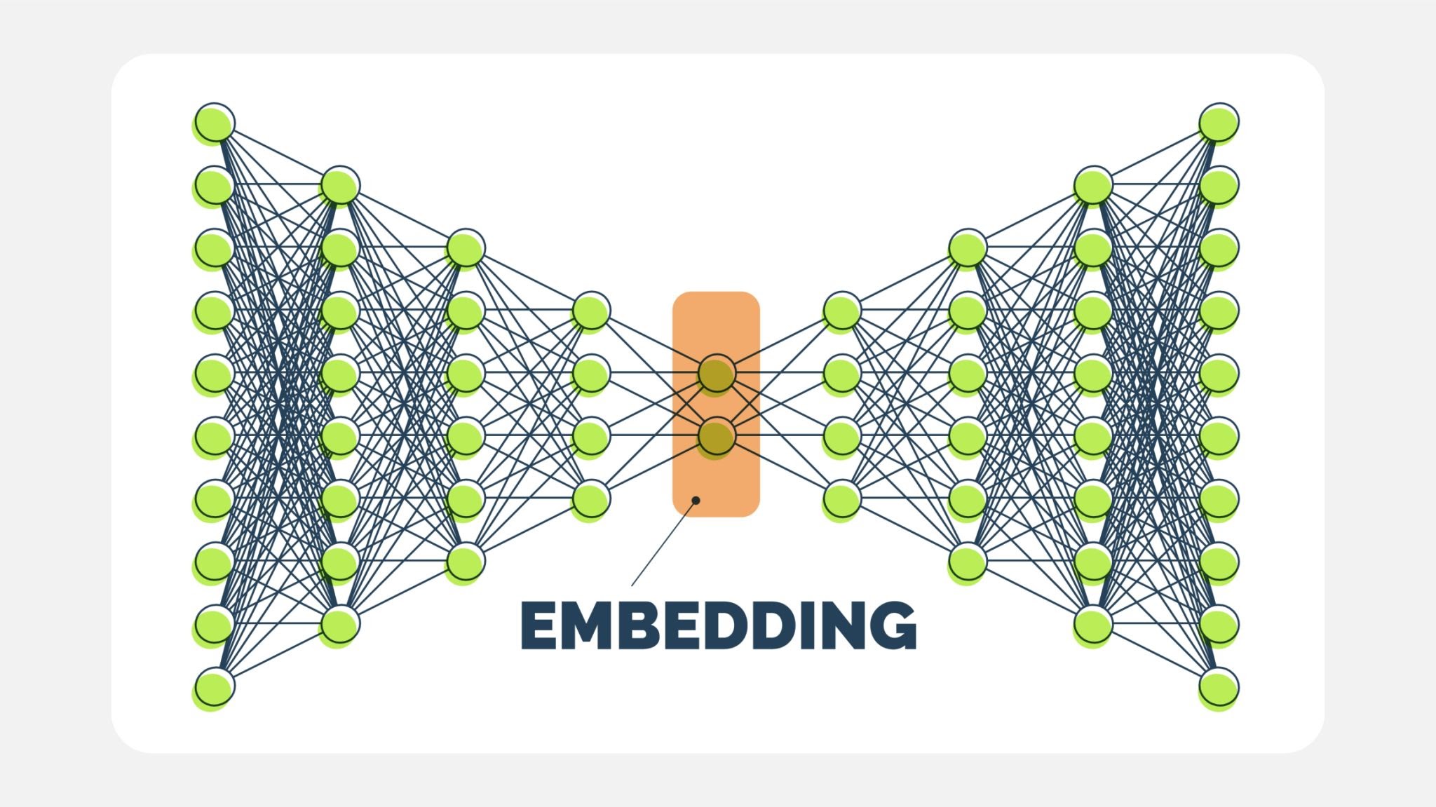
The "Face Embedding" Vector
When we run DeepFace.represent, we are asking the model to convert the face into a mathematical descriptor, often called an Embedding.
- What is it? It is a list of floating-point numbers (e.g., 128, 512, or 4096 numbers, depending on the model).
- The Concept: The network is trained using Triplet Loss. It learns to map face images into a high-dimensional Euclidean space where:
- Distances between images of the same person are small.
- Distances between images of different people are large.
Why is this powerful? We don't need to retrain the model to recognize a new person. We simply calculate their embedding once and store it. To recognize them later, we calculate the embedding of the new face and see if the mathematical distance is close to the stored vector.
$$d(A, B) = || f(A) - f(B) ||_2$$
embedding_objs = DeepFace.represent(astronaut_bgr)
24-09-19 14:18:53 - vgg_face_weights.h5 will be downloaded...
Downloading...
From: https://github.com/serengil/deepface_models/releases/download/v1.0/vgg_face_weights.h5
To: /root/.deepface/weights/vgg_face_weights.h5
100%|██████████| 580M/580M [00:02<00:00, 281MB/s]
print(embedding_objs[0].keys())
print(len(embedding_objs[0]["embedding"]))
dict_keys(['embedding', 'facial_area', 'face_confidence'])
4096
Facial Attribute Analysis
Beyond identity, deep learning models can be trained to classify attributes. DeepFace.analyze does not use the same model as represent. Instead, it runs an ensemble of different models trained on specific datasets:
- Emotion: Typically trained on the FER-2013 dataset. It classifies the face into bins: angry, fear, neutral, sad, disgust, happy, surprise.
- Age: A regression model trained to estimate the apparent age (trained on the IMDB-WIKI dataset).
- Gender: A binary classification model.
- Race): A classification model trained on datasets labeled with ethnicity.
Note on Ethics and Bias: It is crucial to note that attribute analysis models inherit the biases of their training data. If a dataset lacks diversity, the model will perform poorly on underrepresented groups. Additionally, "Race" and "Gender" classification by AI is a subject of significant ethical debate regarding accuracy and social impact.
%%capture
analyze_face = DeepFace.analyze(astronaut_bgr)
analyze_face
[{'emotion': {'angry': 1.1502769095704066e-11,
   'disgust': 6.004073561188443e-22,
   'fear': 2.4250154502244886e-13,
   'happy': 99.26499123960681,
   'sad': 4.274496567241756e-08,
   'surprise': 0.0002363198659508805,
   'neutral': 0.7347721578790044},
  'dominant_emotion': 'happy',
  'region': {'x': 176,
   'y': 66,
   'w': 97,
   'h': 97,
   'left_eye': (247, 103),
   'right_eye': (202, 100)},
  'face_confidence': 0.92,
  'age': 33,
  'gender': {'Woman': 99.80695843696594, 'Man': 0.19304464804008603},
  'dominant_gender': 'Woman',
  'race': {'asian': 0.00044597509258892387,
   'indian': 0.0001380544404128159,
   'black': 2.2719417458461066e-07,
   'white': 98.68490695953369,
   'middle eastern': 0.38867348339408636,
   'latino hispanic': 0.9258316829800606},
'dominant_race': 'white'}] analyze_face[0]['dominant_emotion']
'happy'
Szeliski is a really good resource for today's Colab session. See sections 6.2 and 6.3 for more info.
Intersection Over Union (IoU)
In simple Image Classification, evaluating a model is binary: the model either predicted "Cat" correctly, or it didn't.
However, in Object Detection, the model predicts a bounding box. It is statistically impossible for the model to predict the exact pixel coordinates of the ground truth box. Even a human drawing a box twice will vary slightly.
We need a metric that measures how much the predicted box overlaps with the ground truth. That metric is IoU (also known as the Jaccard Index).
1. The Formula
IoU is a ratio that compares the area where the two boxes overlap against the total area covered by both boxes.
$$IoU = \frac{\text{Area of Intersection}}{\text{Area of Union}}$$
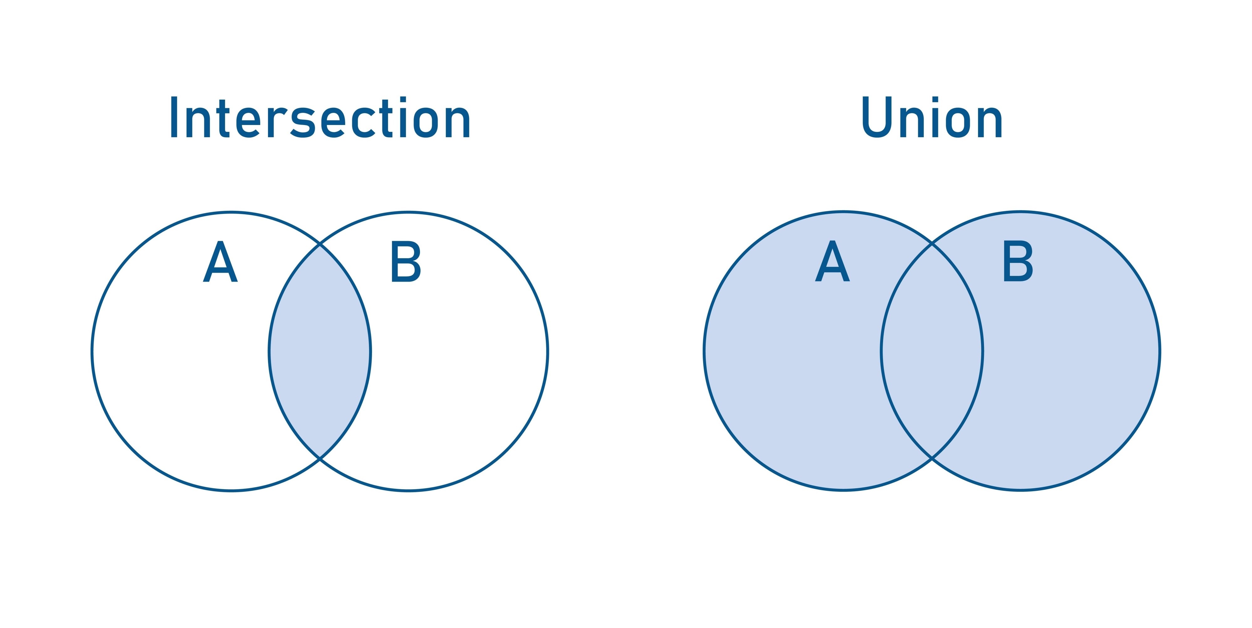
- Intersection: The area where the two boxes overlap (the cyan region in typical diagrams).
- Union: The total area covered by both boxes combined.
- Math Note: $Union = Area_A + Area_B - Intersection$. We subtract the intersection once because it is counted twice (once in $A$ and once in $B$).
2. Why is this important?
IoU is the standard metric for two major tasks:
- Metric for Success: In competitions (like COCO or PASCAL VOC), a prediction is often counted as a True Positive only if the $IoU > 0.5$. If the IoU is $0.4$, the detection is considered a False Positive (a miss), even if the model found the right object.
- Non-Maximum Suppression (NMS): When a model detects the same object multiple times (e.g., 5 boxes around one face), we use IoU to find the overlapping boxes and collapse them into a single best prediction.
3. Interpreting IoU Scores
- IoU = 1.0: Perfect match (Ground truth and Prediction are identical).
- IoU > 0.5: Usually considered a "Good" prediction in standard benchmarks.
- IoU < 0.5: Poor overlap, usually considered a "Miss."
- IoU = 0.0: No overlap at all.
4. Calculating Intersection Coordinates
In the code below, we calculate the intersection rectangle mathematically. Given two boxes, BoxA and BoxB, the intersection rectangle is defined by:
- Top-Left $(x, y)$: The maximum of the top-left coordinates of the two boxes.
- Bottom-Right $(x, y)$: The minimum of the bottom-right coordinates.
If the "max left" is greater than the "min right," the boxes do not overlap.
# Define ground truth and predicted bounding boxes
gt_box = [50, 50, 150, 150]  # [x, y, width, height]
pred_box = [100, 100, 200, 200]  # [x, y, width, height]

fig, ax = plt.subplots(1, figsize=(8, 8))

# Plot ground truth box
gt_rect = patches.Rectangle((gt_box[0], gt_box[1]), gt_box[2], gt_box[3],
                            linewidth=2, edgecolor='blue', facecolor='none', label='Ground Truth')
ax.add_patch(gt_rect)

# Plot predicted box
pred_rect = patches.Rectangle((pred_box[0], pred_box[1]), pred_box[2], pred_box[3],
                              linewidth=2, edgecolor='red', facecolor='none', label='Prediction')
ax.add_patch(pred_rect)

plt.xlabel('X')
plt.ylabel('Y')
plt.title('IoU Visualization')
plt.legend()

# Display the plot
plt.xlim(0, 300)
plt.ylim(0, 300)
plt.gca().set_aspect('equal', adjustable='box')
plt.show()

# Calculate the coordinates of the intersection rectangle
x_left = max(gt_box[0], pred_box[0])
y_top = max(gt_box[1], pred_box[1])
x_right = min(gt_box[0] + gt_box[2], pred_box[0] + pred_box[2])
y_bottom = min(gt_box[1] + gt_box[3], pred_box[1] + pred_box[3])

# Calculate the width and height of the intersection rectangle
intersection_width = max(0, x_right - x_left)
intersection_height = max(0, y_bottom - y_top)

# Calculate the area of intersection
intersection_area = intersection_width * intersection_height

# Calculate the area of the ground truth and predicted boxes
gt_area = gt_box[2] * gt_box[3]
pred_area = pred_box[2] * pred_box[3]

# Calculate the area of union
union_area = gt_area + pred_area - intersection_area

# Calculate IoU
iou = intersection_area / union_area

# Print the IoU
print(f'Intersection Area: {intersection_area}')
print(f'Union Area: {union_area}')
print(f'IoU: {iou}')
Intersection Area: 10000
Union Area: 52500
IoU: 0.19047619047619047